Access the Underlying Data

Setup to make the output clean for the docs:

%%capture
from threeML import silence_logs
import warnings
warnings.filterwarnings("ignore")
silence_logs()
import matplotlib.pyplot as plt
%matplotlib inline
from jupyterthemes import jtplot
jtplot.style(context="talk", fscale=1, ticks=True, grid=False)

Sometime you maybe want to access the underlying data of the analysis to do your own analysis or tests with this data. This section shows how to access some basic quantities, like for example the detected counts per energy channel and the response matrix. First we have to initialize the usual objects in PySPI.

from astropy.time import Time
import numpy as np
from pyspi.utils.function_utils import find_response_version
from pyspi.utils.response.spi_response_data import ResponseDataRMF
from pyspi.utils.response.spi_response import ResponseRMFGenerator
from pyspi.utils.response.spi_drm import SPIDRM
from pyspi.utils.data_builder.time_series_builder import TimeSeriesBuilderSPI
from pyspi.SPILike import SPILikeGRB

grbtime = Time("2012-07-11T02:44:53", format='isot', scale='utc')
ein = np.geomspace(20,800,300)
ebounds = np.geomspace(20,400,30)
version = find_response_version(grbtime)
rsp_base = ResponseDataRMF.from_version(version)
det=0
ra = 94.6783
dec = -70.99905
drm_generator = ResponseRMFGenerator.from_time(grbtime,
                                                det,
                                                ebounds,
                                                ein,
                                                rsp_base)
sd = SPIDRM(drm_generator, ra, dec)
tsb = TimeSeriesBuilderSPI.from_spi_grb(f"SPIDet{det}",
    det,
    grbtime,
    response=sd,
    sgl_type="both",
    )
active_time = "65-75"
bkg_time1 = "-500--10"
bkg_time2 = "150-1000"
tsb.set_active_time_interval(active_time)
tsb.set_background_interval(bkg_time1, bkg_time2)
sl = tsb.to_spectrumlike()
plugin = SPILikeGRB.from_spectrumlike(sl,free_position=False)

Using the irfs that are valid between 10/05/27 12:45:00 and present (YY/MM/DD HH:MM:SS)

In the following it is listed how you can access some of the basic underlying data.

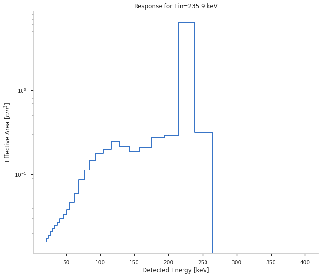
Response Matrix

Get response matrix and plot the response for one incoming energy.

import matplotlib.pyplot as plt
ein_id = 200
matrix = sd.matrix

fig, ax = plt.subplots(1,1)
ax.step(ebounds[1:], matrix[:,ein_id])
ax.set_title(f"Response for Ein={round(ein[ein_id], 1)} keV")
ax.set_xlabel("Detected Energy [keV]")
ax.set_ylabel("Effective Area [$cm^2$]")
ax.set_yscale("log");

Event Data

The data is saved as time tagged events. You can access the arrival time and reconstructed energy bin of every photons. It is important to keep in mind that the reconstructed energy is not the true energy, it is just the energy assigned to one of the energy channels.

#arrival times (time in seconds relative to given trigger time)
arrival_times = tsb.time_series.arrival_times

#energy bin of the events
energy_bin = tsb.time_series.measurement

Lightcurve Data

With the event data you can create the lightcurves manually

# plot lightcurves for all echans summed together
bins = np.linspace(-100,200,300)
cnts, bins = np.histogram(arrival_times, bins=bins)

fig, ax = plt.subplots(1,1)
ax.step(bins[1:], cnts)
ax.set_xlabel("Time [s]")
ax.set_ylabel("Counts [cnts]")
ax.set_title("Lightcurve")
ax.legend();

No handles with labels found to put in legend.

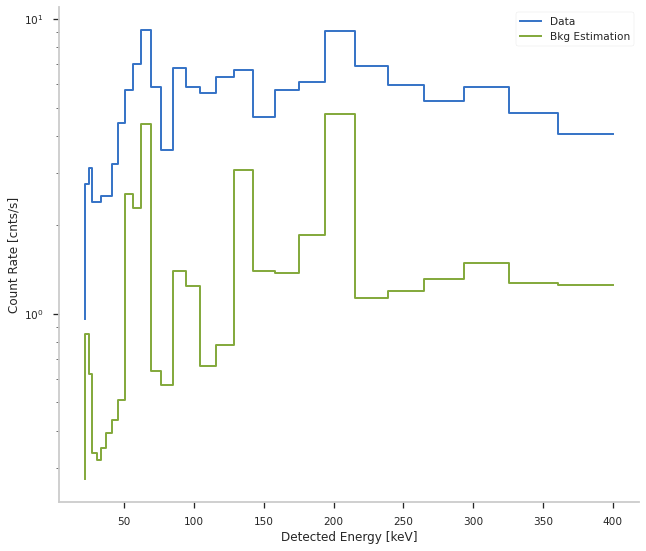
Observed Data Active Time

Get the observed data of the active time and background time selection

# counts
active_time_counts = plugin.observed_counts
estimated_background_counts = plugin.background_counts

# exposure
exposure = plugin.exposure

fig, ax = plt.subplots(1,1)
ax.step(ebounds[1:], active_time_counts/exposure, label="Data")
ax.step(ebounds[1:], estimated_background_counts/exposure, label="Bkg Estimation")

ax.set_xlabel("Detected Energy [keV]")
ax.set_ylabel("Count Rate [cnts/s]")
ax.set_yscale("log")
ax.legend();