Response

Setup to make the output clean for the docs:

%%capture
from threeML import silence_logs
import warnings
warnings.filterwarnings("ignore")
silence_logs()
import matplotlib.pyplot as plt
%matplotlib inline
from jupyterthemes import jtplot
jtplot.style(context="talk", fscale=1, ticks=True, grid=False)

For every analysis of SPI data we need the correct response for the observation, which is the connection between physical spectra and detected counts. Normally the response is a function of the position of the source in the satellite frame, the input energies of the physical spectrum and the output energy bins of the experiment. For SPI, there is also a time dependency, because a few detectors failed during the mission time and this changed the response of the surrounding detectors.

In PySPI we construct the response from the official IRF and RMF files, which we interpolate for a given source position and user chosen input and output energy bins.

We start by defining a time, for which we want to construct the response, to get the pointing information of the satellite at this time and the version number of the response.

from astropy.time import Time
rsp_time = Time("2012-07-11T02:42:00", format='isot', scale='utc')

Next we define the input and output energy bins for the response.

import numpy as np
ein = np.geomspace(20,8000,1000)
ebounds = np.geomspace(20,8000,100)

Get the response version and construct the rsp base, which is an object holding all the information of the IRF and RMF for this response version. We use this, because if we want to combine many observations later, we don’t want to read in this for every observation independently, because this would use a lot of memory. Therefore all the observations with the same response version can share this rsp_base object.

from pyspi.utils.function_utils import find_response_version
from pyspi.utils.response.spi_response_data import ResponseDataRMF
version = find_response_version(rsp_time)
print(version)
rsp_base = ResponseDataRMF.from_version(version)

4
Using the irfs that are valid between 10/05/27 12:45:00 and present (YY/MM/DD HH:MM:SS)

Now we can construct the response for a given detector and source position (in ICRS coordinates)

from pyspi.utils.response.spi_response import ResponseRMFGenerator
from pyspi.utils.response.spi_drm import SPIDRM
det = 0
ra = 94.6783
dec = -70.99905
drm_generator = ResponseRMFGenerator.from_time(rsp_time,
                                                det,
                                                ebounds,
                                                ein,
                                                rsp_base)
sd = SPIDRM(drm_generator, ra, dec)

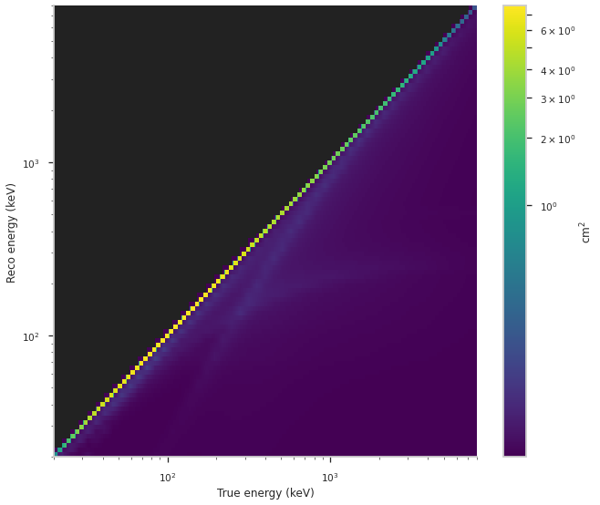
SPIDRM is a child class of InstrumentResponse from threeML, therefore we can use the plotting functions from 3ML.

fig = sd.plot_matrix()