Analyse GRB data
Setup to make the output clean for the docs:
[1]:
%%capture
from threeML import silence_logs
import warnings
warnings.filterwarnings("ignore")
silence_logs()
import matplotlib.pyplot as plt
%matplotlib inline
from jupyterthemes import jtplot
jtplot.style(context="talk", fscale=1, ticks=True, grid=False)
The first thing we need to do, is to specify the time of the GRB. We do this by specifying a astropy time object or a string in the format YYMMDD HHMMSS.
[2]:
from astropy.time import Time
grbtime = Time("2012-07-11T02:44:53", format='isot', scale='utc')
#grbtime = "120711 024453" # works also
Next, we need to specify the output and input energy bins we want to use.
[3]:
import numpy as np
ein = np.geomspace(20,800,300)
ebounds = np.geomspace(20,400,30)
Due to detector failures there are several versions of the response for SPI. Therefore we have to find the version number for the time of the GRB and construct the base response object for this version.
[4]:
from pyspi.utils.function_utils import find_response_version
from pyspi.utils.response.spi_response_data import ResponseDataRMF
version = find_response_version(grbtime)
print(version)
rsp_base = ResponseDataRMF.from_version(version)
4
Using the irfs that are valid between 10/05/27 12:45:00 and present (YY/MM/DD HH:MM:SS)
Now we can create the response object for detector 0 and set the position of the GRB, which we already know.
[5]:
from pyspi.utils.response.spi_response import ResponseRMFGenerator
from pyspi.utils.response.spi_drm import SPIDRM
det=0
ra = 94.6783
dec = -70.99905
drm_generator = ResponseRMFGenerator.from_time(grbtime,
                                                det,
                                                ebounds,
                                                ein,
                                                rsp_base)
sd = SPIDRM(drm_generator, ra, dec)
With this we can build a time series and we use all the single events in this case (PSD + non PSD; see section about electronic noise). To be able to convert the time series into 3ML plugins later, we need to assign them a response object.
[6]:
from pyspi.utils.data_builder.time_series_builder import TimeSeriesBuilderSPI
tsb = TimeSeriesBuilderSPI.from_spi_grb(f"SPIDet{det}",
    det,
    grbtime,
    response=sd,
    sgl_type="both",
    )
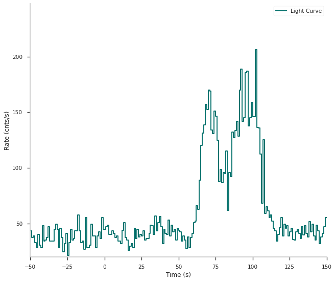
Now we can have a look at the light curves from -50 to 150 seconds around the specified GRB time.
[7]:
fig = tsb.view_lightcurve(-50,150)
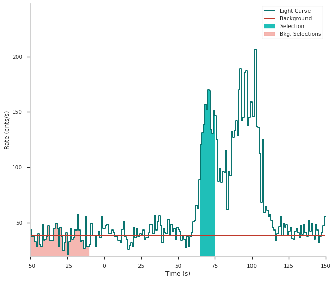
With this we can select the active time and some background time intervals.
[8]:
active_time = "65-75"
bkg_time1 = "-500--10"
bkg_time2 = "150-1000"
tsb.set_active_time_interval(active_time)
tsb.set_background_interval(bkg_time1, bkg_time2)
We can check if the selection and background fitting worked by looking again at the light curve
[9]:
fig = tsb.view_lightcurve(-50,150)
For the fit we of course want to use all the available detectors. So we first check which detectors were still working at that time.
[10]:
from pyspi.utils.livedets import get_live_dets
active_dets = get_live_dets(time=grbtime, event_types=["single"])
print(active_dets)
[ 0 3 4 6 7 8 9 10 11 12 13 14 15 16 18]
Now we loop over these detectors, build the times series, fit the background and construct the SPILikeGRB plugins which we can use in 3ML.
[11]:
from pyspi.SPILike import SPILikeGRB
from threeML import DataList
spilikes = []
for d in active_dets:
    drm_generator = ResponseRMFGenerator.from_time(grbtime,
                                                    d,
                                                    ebounds,
                                                    ein,
                                                    rsp_base)
    sd = SPIDRM(drm_generator, ra, dec)
    tsb = TimeSeriesBuilderSPI.from_spi_grb(f"SPIDet{d}",
                                                d,
                                                grbtime,
                                                response=sd,
                                                sgl_type="both",
                                                )
    tsb.set_active_time_interval(active_time)
    tsb.set_background_interval(bkg_time1, bkg_time2)

    sl = tsb.to_spectrumlike()
    spilikes.append(SPILikeGRB.from_spectrumlike(sl,
                                                free_position=False))
datalist = DataList(*spilikes)
Now we have to specify a model for the fit. We use astromodels for this.
[12]:
from astromodels import *
pl = Powerlaw()
pl.K.prior = Log_uniform_prior(lower_bound=1e-6, upper_bound=1e4)
pl.K.bounds = (1e-6, 1e4)
pl.index.set_uninformative_prior(Uniform_prior)
pl.piv.value = 200
ps = PointSource('GRB',ra=ra, dec=dec, spectral_shape=pl)

model = Model(ps)
Everything is ready to fit now! We make a Bayesian fit here with emcee
[13]:
from threeML import BayesianAnalysis
ba_spi = BayesianAnalysis(model, datalist)
ba_spi.set_sampler("emcee", share_spectrum=True)
ba_spi.sampler.setup(n_walkers=20, n_iterations=500)
ba_spi.sample()
Maximum a posteriori probability (MAP) point:
| result | unit | |
|---|---|---|
| parameter | ||
| GRB.spectrum.main.Powerlaw.K | (2.25 +/- 0.04) x 10^-2 | 1 / (cm2 keV s) |
| GRB.spectrum.main.Powerlaw.index | -1.014 -0.018 +0.017 |
Values of -log(posterior) at the minimum:
| -log(posterior) | |
|---|---|
| SPIDet0 | -79.708463 |
| SPIDet10 | -64.725855 |
| SPIDet11 | -68.904660 |
| SPIDet12 | -68.001808 |
| SPIDet13 | -83.540126 |
| SPIDet14 | -73.634753 |
| SPIDet15 | -62.837192 |
| SPIDet16 | -62.263356 |
| SPIDet18 | -75.559807 |
| SPIDet3 | -72.583142 |
| SPIDet4 | -73.741573 |
| SPIDet6 | -59.864307 |
| SPIDet7 | -78.342385 |
| SPIDet8 | -60.375355 |
| SPIDet9 | -59.532740 |
| total | -1043.615524 |
Values of statistical measures:
| statistical measures | |
|---|---|
| AIC | 2091.258825 |
| BIC | 2099.381739 |
| DIC | 2137.264487 |
| PDIC | 1.935718 |
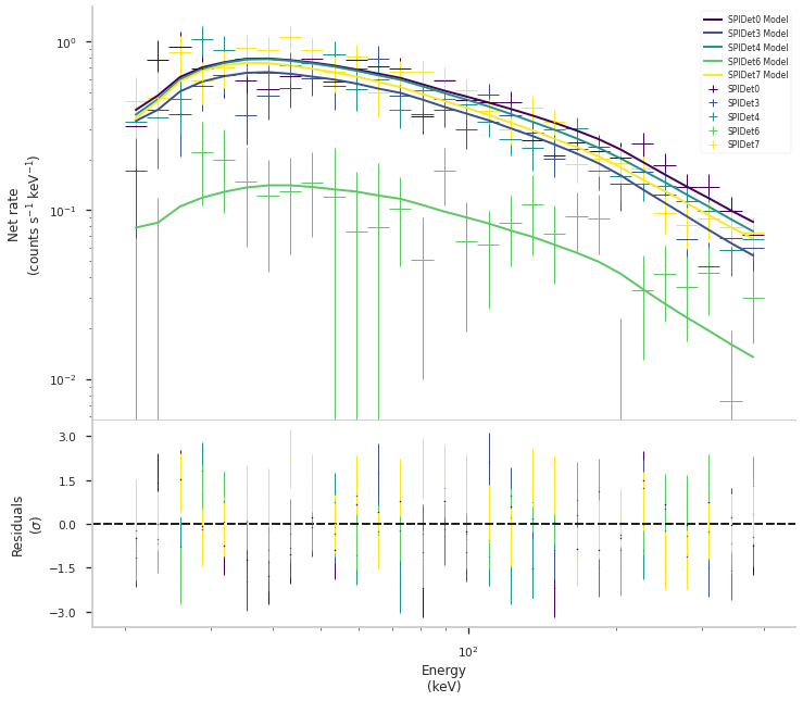
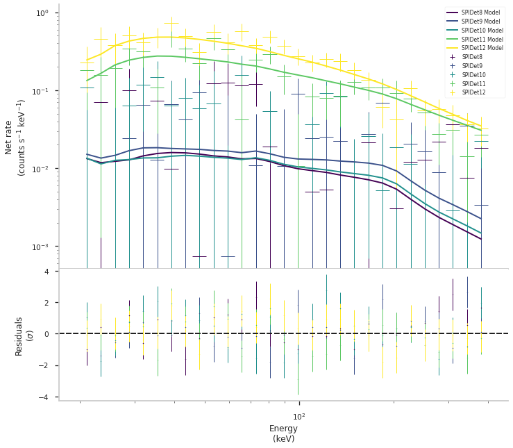
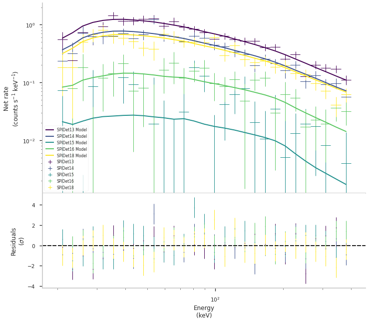
We can inspect the fits with residual plots
[14]:
from threeML import display_spectrum_model_counts
fig = display_spectrum_model_counts(ba_spi,
                                data_per_plot=5,
                                source_only=True,
                                show_background=False,
                                model_cmap="viridis",
                                data_cmap="viridis",
                                background_cmap="viridis")
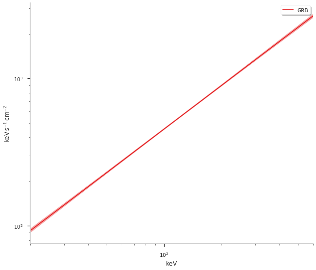
and have a look at the spectrum
[15]:
from threeML import plot_spectra
fig = plot_spectra(ba_spi.results, flux_unit="keV/(s cm2)", ene_min=20, ene_max=600)
We can also get a summary of the fit and write the results to disk (see 3ML documentation).
It is also possible to localize GRBs with PySPI, to this we simply free the position of point source with:
[16]:
for s in spilikes:
    s.set_free_position(True)
datalist = DataList(*spilikes)
Initialize the Bayesian Analysis and start the sampling with MultiNest. To use MultiNest you need to install pymultinest according to its documentation.
[17]:
import os
os.mkdir("./chains_grb_example")
ba_spi = BayesianAnalysis(model, datalist)
ba_spi.set_sampler("multinest")
ba_spi.sampler.setup(500,
                    chain_name='./chains_grb_example/docsfit1_',
                    resume=False,
                    verbose=False)
ba_spi.sample()
Freeing the position of SPIDet0 and setting priors
Freeing the position of SPIDet3 and setting priors
Freeing the position of SPIDet4 and setting priors
Freeing the position of SPIDet6 and setting priors
Freeing the position of SPIDet7 and setting priors
Freeing the position of SPIDet8 and setting priors
Freeing the position of SPIDet9 and setting priors
Freeing the position of SPIDet10 and setting priors
Freeing the position of SPIDet11 and setting priors
Freeing the position of SPIDet12 and setting priors
Freeing the position of SPIDet13 and setting priors
Freeing the position of SPIDet14 and setting priors
Freeing the position of SPIDet15 and setting priors
Freeing the position of SPIDet16 and setting priors
Freeing the position of SPIDet18 and setting priors
 *****************************************************
 MultiNest v3.12
 Copyright Farhan Feroz & Mike Hobson
 Release Nov 2019

 no. of live points =  500
 dimensionality =    4
 *****************************************************
  analysing data from chains_grb_example/docsfit1_.txt ln(ev)=  -1088.6098789639104      +/-  0.21907028375800258

 Total Likelihood Evaluations:       291325
 Sampling finished. Exiting MultiNest
Maximum a posteriori probability (MAP) point:
| result | unit | |
|---|---|---|
| parameter | ||
| GRB.position.ra | (9.466 +/- 0.007) x 10 | deg |
| GRB.position.dec | (-7.1053 -0.0017 +0.0016) x 10 | deg |
| GRB.spectrum.main.Powerlaw.K | (2.27 +/- 0.04) x 10^-2 | 1 / (cm2 keV s) |
| GRB.spectrum.main.Powerlaw.index | -1.014 -0.017 +0.018 |
Values of -log(posterior) at the minimum:
| -log(posterior) | |
|---|---|
| SPIDet0 | -81.578248 |
| SPIDet10 | -67.160529 |
| SPIDet11 | -71.383255 |
| SPIDet12 | -69.645227 |
| SPIDet13 | -86.448622 |
| SPIDet14 | -76.474985 |
| SPIDet15 | -65.363899 |
| SPIDet16 | -64.161539 |
| SPIDet18 | -77.792754 |
| SPIDet3 | -76.674979 |
| SPIDet4 | -73.979425 |
| SPIDet6 | -62.198945 |
| SPIDet7 | -78.372394 |
| SPIDet8 | -62.911150 |
| SPIDet9 | -62.034177 |
| total | -1076.180129 |
Values of statistical measures:
| statistical measures | |
|---|---|
| AIC | 2160.453280 |
| BIC | 2176.661641 |
| DIC | 2134.789897 |
| PDIC | 3.876941 |
| log(Z) | -472.777263 |
We can use the 3ML features to create a corner plot for this fit:
[18]:
from threeML.config.config import threeML_config
threeML_config.bayesian.corner_style.show_titles = False
fig = ba_spi.results.corner_plot(components=["GRB.position.ra", "GRB.position.dec"])
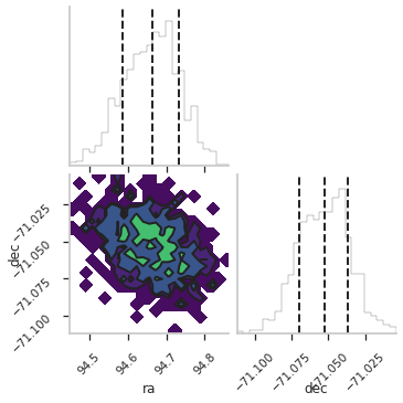
When we compare the results for ra and dec, we can see that this matches with the position from Swift-XRT for the same GRB (RA, Dec = 94.67830, -70.99905)