Electronic Noise Region

Setup to make the output clean for the docs:

%%capture
from threeML import silence_logs
import warnings
warnings.filterwarnings("ignore")
silence_logs()
import matplotlib.pyplot as plt
%matplotlib inline
from jupyterthemes import jtplot
jtplot.style(context="talk", fscale=1, ticks=True, grid=False)

Since shortly after the launch of INTEGRAL it is known that there are spurious events in the SPI data around ~1.5 MeV. A paper from Roques & Jourdain gives an explanation for this problem. Luckily this problem exists only in the events that only triggered the analog front-end electronics (AFEE). The events that trigger in addition the pulse shape discrimination electronics (PSD) do not show this problem. According to Roques & Jourdain, one should therefore use the PSD events whenever this is possible, which is for events between ~500 and 2500 keV (the precise boundaries were changed during the mission a few times). In the following the events that trigger both the AFEE and PSD are called “PSD events” and the other normal “single events” or “Non-PSD events”, even thought the PSD events are of course also single events.

To account for this problem in our analysis we can construct plugins for the “PSD events” and the for the “Non-PSD events” and use only the events with the correct flags, when we construct the time series.

Let’s check the difference between the PSD and the Non-PSD events, to see the effect in real SPI data.

First we define the time and the energy bins we want to use. Then we construct the time series for the three cases:

1. Only the events that trigger AFEE and not PSD

2. Only the events that trigger AFEE and PSD

3. All the single events

from astropy.time import Time
import numpy as np
from pyspi.utils.data_builder.time_series_builder import TimeSeriesBuilderSPI
grbtime = Time("2012-07-11T02:44:53", format='isot', scale='utc')
ebounds = np.geomspace(20,8000,300)
det = 0

from pyspi.utils.data_builder.time_series_builder import TimeSeriesBuilderSPI
tsb_sgl = TimeSeriesBuilderSPI.from_spi_grb(f"SPIDet{det}",
    det,
    grbtime,
    ebounds=ebounds,
    sgl_type="sgl",
    )

tsb_psd = TimeSeriesBuilderSPI.from_spi_grb(f"SPIDet{det}",
    det,
    grbtime,
    ebounds=ebounds,
    sgl_type="psd",
    )

tsb_both = TimeSeriesBuilderSPI.from_spi_grb(f"SPIDet{det}",
    det,
    grbtime,
    ebounds=ebounds,
    sgl_type="both",
    )

We can check the light curves for all three cases.

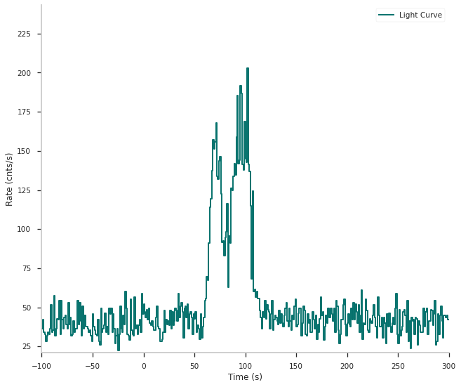
print("Only AFEE:")
fig = tsb_sgl.view_lightcurve(-100,300)

Only AFEE:

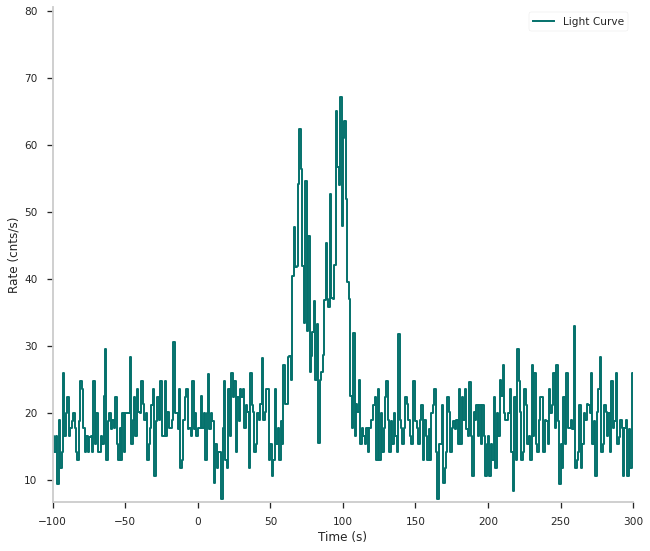
print("AFFE and PSD trigger:")
fig = tsb_psd.view_lightcurve(-100,300)

AFFE and PSD trigger:

print("Both Combined:")
fig = tsb_both.view_lightcurve(-100,300)

Both Combined:

We can see that the PSD event light curve has way less counts. This is due to the fact, that the PSD trigger only starts detecting photons with energies >~ 400 keV.

Next we can get the time integrated counts per energy channel.

tstart = -500
tstop = 1000
counts_sgl = tsb_sgl.time_series.count_per_channel_over_interval(tstart, tstop)
counts_psd = tsb_psd.time_series.count_per_channel_over_interval(tstart, tstop)
counts_both = tsb_both.time_series.count_per_channel_over_interval(tstart, tstop)

We can now plot the counts as a function of the energy channel energies

import matplotlib.pyplot as plt
fig, ax = plt.subplots(1,1)
ax.step(ebounds[1:], counts_sgl, label="Only AFEE")
ax.step(ebounds[1:], counts_psd, label="AFEE and PSD")
ax.step(ebounds[1:], counts_both, label="All")
ax.set_xlabel("Detected Energy [keV]")
ax.set_ylabel("Counts")
ax.set_xlim(20,3500)
ax.set_yscale("log")
ax.legend();

Several features are visible.

1. A sharp cutoff at small energies for the PSD events, which is due to the low energy threshold in the PSD electronics.

2. For energies>~2700 keV the PSD events decrease again faster than the other events.

3. In the Non-PSD events we see a peak at ~ 1600 keV that is not visible in the PSD events. This is the so called electronic noise, which consists of spurious events.

4. The fraction of PSD events to all single events between ~500 and ~2700 keV is very stable and can be explained by an additional dead time for the PSD electronics.