Fit for the PSD Efficiency
Setup to make the output clean for the docs:
[1]:
%%capture
from threeML import silence_logs
import warnings
warnings.filterwarnings("ignore")
silence_logs()
import matplotlib.pyplot as plt
%matplotlib inline
from jupyterthemes import jtplot
jtplot.style(context="talk", fscale=1, ticks=True, grid=False)
The first thing we need to do, is to specify the time of the GRB. We do this by specifying a astropy time object or a string in the format YYMMDD HHMMSS.
[2]:
from astropy.time import Time
grbtime = Time("2012-07-11T02:44:53", format='isot', scale='utc')
#grbtime = "120711 024453" # works also
Now we want to analyze in total the energy between 20 and 2000 keV. So we have to take into account the spurious events in the Non-PSD events (see electronic noise section). For the energy bins up to 500 keV we will use all the single events and from 500 to 2000 keV, we will only use the PSD events.
[3]:
import numpy as np
ein = np.geomspace(20,3000,300)
ebounds_sgl = np.geomspace(20,500,30)
ebounds_psd = np.geomspace(500,2000,30)
Due to detector failures there are several versions of the response for SPI. Therefore we have to find the version number for the time of the GRB and construct the base response object for this version.
[4]:
from pyspi.utils.function_utils import find_response_version
from pyspi.utils.response.spi_response_data import ResponseDataRMF
version = find_response_version(grbtime)
print(version)
rsp_base = ResponseDataRMF.from_version(version)
4
Using the irfs that are valid between 10/05/27 12:45:00 and present (YY/MM/DD HH:MM:SS)
Now we can create the response object for detector 0 and set the position of the GRB, which we already know.
[5]:
from pyspi.utils.response.spi_response import ResponseRMFGenerator
from pyspi.utils.response.spi_drm import SPIDRM
det=0
ra = 94.6783
dec = -70.99905
drm_generator_sgl = ResponseRMFGenerator.from_time(grbtime,
                                                    det,
                                                    ebounds_sgl,
                                                    ein,
                                                    rsp_base)
sd_sgl = SPIDRM(drm_generator_sgl, ra, dec)
With this we can build a time series and we use all the single events in this case (PSD + non PSD; see section about electronic noise). To be able to convert the time series into 3ML plugins later, we need to assign them a response object.
[6]:
from pyspi.utils.data_builder.time_series_builder import TimeSeriesBuilderSPI
tsb_sgl = TimeSeriesBuilderSPI.from_spi_grb(f"SPIDet{det}",
                                            det,
                                            grbtime,
                                            response=sd_sgl,
                                            sgl_type="both",
                                            )
Now we can have a look at the light curves from -50 to 150 seconds around the specified GRB time.
[7]:
fig = tsb_sgl.view_lightcurve(-50,150)

With this we can select the active time and some background time intervals.
[8]:
active_time = "65-75"
bkg_time1 = "-500--10"
bkg_time2 = "150-1000"
tsb_sgl.set_active_time_interval(active_time)
tsb_sgl.set_background_interval(bkg_time1, bkg_time2)
We can check if the selection and background fitting worked by looking again at the light curve
[9]:
fig = tsb_sgl.view_lightcurve(-50,150)

In this example we use three detectors (IDs: 0, 3 and 4). For these three detectors we build the times series, fit the background and construct the SPILikeGRB plugins which we can use in 3ML.
[10]:
from pyspi.SPILike import SPILikeGRB
from threeML import DataList
spilikes_sgl = []
spilikes_psd = []
for d in [0,3,4]:
    drm_generator_sgl = ResponseRMFGenerator.from_time(grbtime,
                                                        d,
                                                        ebounds_sgl,
                                                        ein,
                                                        rsp_base)
    sd_sgl = SPIDRM(drm_generator_sgl, ra, dec)
    tsb_sgl = TimeSeriesBuilderSPI.from_spi_grb(f"SPIDet{d}",
                                                d,
                                                grbtime,
                                                response=sd_sgl,
                                                sgl_type="both",
                                                )
    tsb_sgl.set_active_time_interval(active_time)
    tsb_sgl.set_background_interval(bkg_time1, bkg_time2)

    sl_sgl = tsb_sgl.to_spectrumlike()
    spilikes_sgl.append(SPILikeGRB.from_spectrumlike(sl_sgl,
                                                    free_position=False))

    drm_generator_psd = ResponseRMFGenerator.from_time(grbtime,
                                                        d,
                                                        ebounds_psd,
                                                        ein,
                                                        rsp_base)
    sd_psd = SPIDRM(drm_generator_psd, ra, dec)
    tsb_psd = TimeSeriesBuilderSPI.from_spi_grb(f"SPIDetPSD{d}",
                                                d,
                                                grbtime,
                                                response=sd_psd,
                                                sgl_type="both",
                                                )
    tsb_psd.set_active_time_interval(active_time)
    tsb_psd.set_background_interval(bkg_time1, bkg_time2)

    sl_psd = tsb_psd.to_spectrumlike()
    spilikes_psd.append(SPILikeGRB.from_spectrumlike(sl_psd,
                                                    free_position=False))

datalist = DataList(*spilikes_sgl, *spilikes_psd)
Now we set a nuisance parameter for the 3ML fit. Nuisance parameter are parameters that only affect one plugin. In this case it is the PSD efficiency for every plugin that uses only PSD events. We do not link the PSD efficiencies in this case, so we determine the PSD efficiency per detector.
[11]:
for i, s in enumerate(spilikes_psd):
    s.use_effective_area_correction(0,1)
Now we have to specify a model for the fit. We use astromodels for this.
[12]:
from astromodels import *
band = Band()
band.K.prior = Log_uniform_prior(lower_bound=1e-6, upper_bound=1e4)
band.K.bounds = (1e-6, 1e4)
band.alpha.set_uninformative_prior(Uniform_prior)
band.beta.set_uninformative_prior(Uniform_prior)
band.xp.prior = Uniform_prior(lower_bound=10,upper_bound=8000)
band.piv.value = 200
ps = PointSource('GRB',ra=ra, dec=dec, spectral_shape=band)

model = Model(ps)
Everything is ready to fit now! We make a Bayesian fit here with MultiNest. To use MultiNest you need to install pymultinest according to its documentation.
[13]:
from threeML import BayesianAnalysis
import os
os.mkdir("./chains_psd_eff")
ba_spi = BayesianAnalysis(model, datalist)
for i, s in enumerate(spilikes_psd):
    s.use_effective_area_correction(0,1)
ba_spi.set_sampler("multinest")

ba_spi.sampler.setup(500,
                    chain_name='./chains_psd_eff/docsfit1_',
                    resume=False,
                    verbose=False)
ba_spi.sample()
 *****************************************************
 MultiNest v3.12
 Copyright Farhan Feroz & Mike Hobson
 Release Nov 2019

 no. of live points =  500
 dimensionality =    7
 *****************************************************
  analysing data from chains_psd_eff/docsfit1_.txt ln(ev)=  -382.17785337379030      +/-  0.15332793358616456
 Total Likelihood Evaluations:        19921
 Sampling finished. Exiting MultiNest

Maximum a posteriori probability (MAP) point:
| result | unit | |
|---|---|---|
| parameter | ||
| GRB.spectrum.main.Band.K | (2.02 +/- 0.08) x 10^-2 | 1 / (cm2 keV s) |
| GRB.spectrum.main.Band.alpha | -1.052 -0.034 +0.033 | |
| GRB.spectrum.main.Band.xp | (5.1 +/- 1.9) x 10^3 | keV |
| GRB.spectrum.main.Band.beta | -3.3 +/- 1.2 | |
| cons_SPIDetPSD0 | (5.4 +/- 0.7) x 10^-1 | |
| cons_SPIDetPSD3 | (6.5 +/- 1.0) x 10^-1 | |
| cons_SPIDetPSD4 | (6.1 +/- 0.9) x 10^-1 |
Values of -log(posterior) at the minimum:
| -log(posterior) | |
|---|---|
| SPIDet0 | -80.155176 |
| SPIDet3 | -77.061524 |
| SPIDet4 | -72.049594 |
| SPIDetPSD0 | -48.358257 |
| SPIDetPSD3 | -39.201423 |
| SPIDetPSD4 | -40.868095 |
| total | -357.694068 |
Values of statistical measures:
| statistical measures | |
|---|---|
| AIC | 730.062835 |
| BIC | 751.501524 |
| DIC | 742.371506 |
| PDIC | 4.881625 |
| log(Z) | -165.977733 |
We can use the 3ML features to create a corner plot for this fit:
[14]:
from threeML.config.config import threeML_config
threeML_config.bayesian.corner_style.show_titles = False
fig = ba_spi.results.corner_plot(components=["cons_SPIDetPSD0", "cons_SPIDetPSD3", "cons_SPIDetPSD4"])
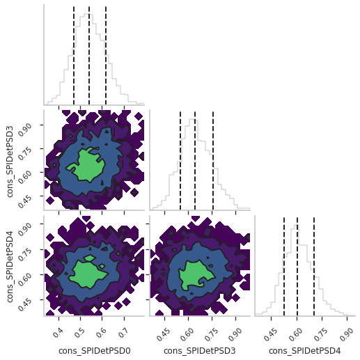
So we see we have a PSD efficiency of ~60 +/- 10 % in this case.